Curve-Generator
The function block creates a customized curve, that is composed of segments based on linear, sine, exponential and logarithm functions.
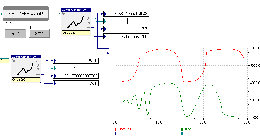
The Curve-Generator is controlled by the commands given at the input “Mode” (see Signals). If the Start command (1) is given, the random parameters of the curve are calculated. The start value of the curve is written to the output “Signal” and the output “State” switches to “Busy”. The time stamp at the output “TimePos” is reset to 0 and the output “Length” provides the duration of the curve in seconds.
If the Run command (2) is given in the next program processing cycle, the time stamp at the output “TimePos” is increased by the time difference between the last two calls of the function block. The according curve value is calculated and written to the “Signal” output.
With the Stop command (0) the curve calculation is stopped for one processing cycle. Subsequently, the calculation can be proceeded with Run or be reinitialized with Start or be paused further cycles with a continuing Stop. After the curve has been ran through, the calculation is finished. The output “State” changes to “Ready” and the value at “TimePos” matches with the duration at “Length”.
After that, the generator can be reinitialized with the Start command and the curve can be output with Run once again. A permanent repeating of the curve can be automated by the Cycle command (3).
The random curve parameters are only recalculated when changing from another command to Start.
The random curve parameters are only recalculated when changing the command to Start. If the Start command is still given for the next processing cycles, they remain unchanged.
Parameters
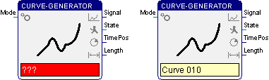
The curve is defined and assigned to the block in the parameter dialog. The dialog can be called during edit or run mode. The name of the assigned curve is displayed in the text field on the function block symbol. A red text field indicates a missing or invalid curve assignment.
Signals
| Name | I/O | Type(s) | Function |
|---|---|---|---|
| Mode | I | WORD | Commands: 0 – Stop 1 – Start 2 – Run 3 – Cycle |
| Signal | O | DOUBLE | Current curve value |
| State | O | WORD | State: 0 – Ready 1 – Busy -1 – Error |
| TimePos | O | DOUBLE | Time stamp in [s] |
| Length | O | DOUBLE | Duration of the curve in [s] |
Example
Curve definition
The parameter dialog of the Curve-Generator block contains the list of all defined curves.
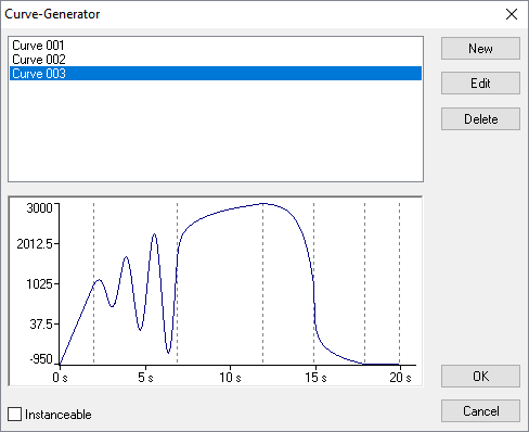
The curves are sorted according to their names. Using the buttons right beside the list, a new curve can be added or the selected one can be edited or deleted. The selected curve is displayed below the list and is assigned to the block when closing the dialog with OK.
When pressing Cancel, the block keeps its original curve assignment. However, changes at the curve definitions are not undone with Cancel.
With the check box in the down left corner, the user can determine in edit mode, whether the curve assignment should be instanceable. That means, that it is possible to assign different curves to the instances of the function block in run mode.
The following dialog for the curve definition is opened with the buttons “Edit” and “New”. The curve name is entered in the upper edit line.
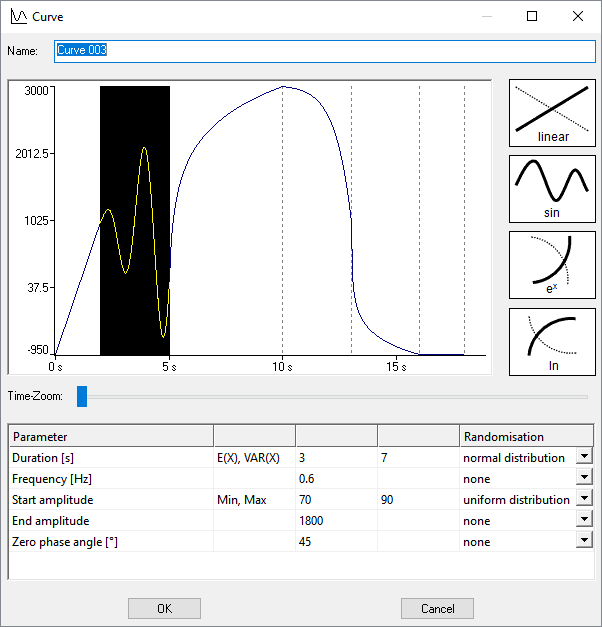
The curve consists of one or more segments. These segments are based on linear, sine, exponential or logarithm functions. To add another segment, one of the four function icons on the right have to be clicked with the left mouse button and dragged into the curve field. Depending on the position of the icon when releasing the mouse button, the new segment is inserted before the first, after the last or between two already existing segments. The new segment is initialized with default parameters and selected.
The selection can easily be changed with the cursor keys or by clicking on another segment. If a segment is clicked with the right mouse button, the belonging context menu opens. The segment can be deleted with the contained command. Alternatively, the selected segment can also be removed by pressing the “Del” key.
The slider below the curve section changes the resolution of the time axis, so small segments can be selected more easily and details are more visible.
The parameters of the selected segment are listed in the table below the curve. The parameters are constants or random numbers. Uniformly distributed random numbers are defined by intervals with minimum and maximum. The expected value E(X) and the variance VAR(X) have to be specified for normally distributed random numbers. The random number types are selected in the drop-lists in the last column of the table. Segments with random parameters are displayed with their expected values in the curve field.
The end value of the curve in a segment is the start value of the next segment. Therefore, the start value is only specified for the first segment. The duration is specified for every segment. The minimum duration is 0.001s and the maximum duration is 3600s. The following table contains additional parameters for the segment types.
| Linear | End value | All values between -1^300 and 1^300 can be specified. |
|---|---|---|
| Sinus | Frequency [Hz] | Frequencies between 1^-10 Hz and 1000 Hz can be entered. |
| Start amplitude End amplitude |
All values between 0 and 1^300 can be specified. | |
| Zero phase angle [°] | The curve calculation in the sine segment starts with the zero-phase angle. It allows to begin with a downward oscillation. Values between 0° and 360° can be specified. | |
| Natural Logarithm | End value | All values between -1^300 and 1^300 can be specified. |
| Supporting point - time [%] Supporting point - value [%] |
Besides the start and end value, the curve is defined by a supporting point. It is displayed in a selected logarithmical segment by crosshairs. At upward trend, the supporting point indicates by how many percent the value has risen over the given percentage of the duration. At downward trend, it defines by how many percent the value has fallen over the given percentage of the duration. Values between 0.1% and 99.9% can be specified. The percentage for the time can only be less than or equal to the percentage for the value. Due to numerical problems in the calculation of the curve, the maximum value percentage can be reduced to up to 99% for smaller time portions. | |
| Exponential | End value | All values between -1^300 and 1^300 can be specified. |
| Supporting point - time [%] Supporting point - value [%] |
In addition to the start and end values, the curve is defined by a supporting point. It is displayed in a selected exponential segment by crosshairs. At upward trend, the supporting point indicates by how many percent the value has risen over the given percentage of the duration. At downward trend, it defines by how many percent the value has fallen over the given percentage of the duration. Values between 0.1% and 99.9% can be specified. The percentage for the value can only be less than or equal to the percentage for the time. Due to numerical problems in the calculation of the curve, the maximum time percentage can be reduced to up to 99% for smaller value portions. |